The Export function will allow you to view recorded data into third party data analysis programs such as Excel, SigmaPlot, or MATLAB, and contains many options to best fit your data needs.

To Export Raw Data:

1. Open the test that contains the data you wish to export 

2. Click on Export at the bottom of the screen to open a pop-out menu

3. From this pop-out menu, choose which tables to export – see image below for explanation of different table options

Note that when exporting to Excel, it's best to use either:

• Tab Separator and a .txt file extension, or
• Comma Separator and file type .csv

4. Click Browse to select the save location, enter a file name, and choose file type. Save as type .csv to open the data with Excel. Click OK

5. When done, click Export 

Explore export options:  

Your export options are listed in this pop-out menu. Notice the three major sections: Export, Include All, and Data Columns.

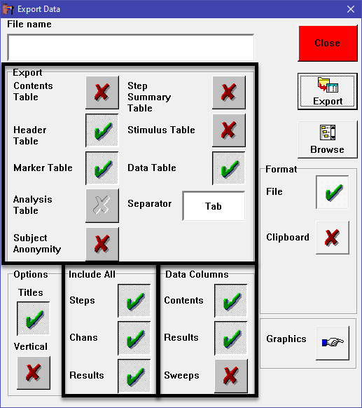
Export:

Here's a table of all of our export options - see examples below.

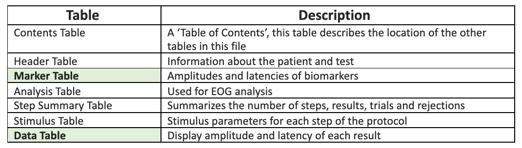
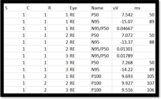
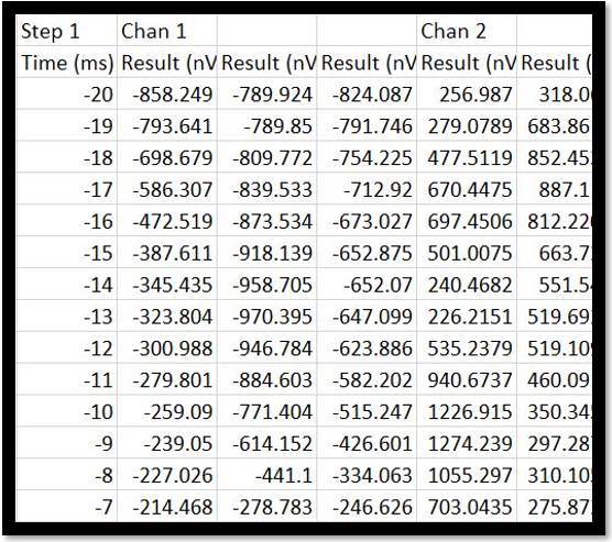
Two of the most common export tables are Data and Marker. Data tables are best for re-graphing results using another software program, while Marker tables are the simplest way to read all biomarker values. 

Include All: 

You may choose to include Steps, Channels, and Results. Each Step of a protocol features different stimulus parameters. Channel refers to a recording from which the data is flowing; this can be RE, LE, occipital lobe, or a virtual channel based on one of these. Results are recorded waveforms that are averages of multiple sweeps.  

Data Columns:  

Pertaining specifically to the Data Table, Contents label the columns, Results show each recorded result, Sweeps display each sweep averaged to create a result. Generally, contents will always be on and sweeps usually shows too much information.  

Examples of each table:  

Marker Table:  

Amplitudes and latencies of biomarkers. S, C, R stand for Step, Channel, Result. Marker Name, amplitude (vU) and latency (ms) are listed.  

Data Table:  

This table lists the amplitude for each datapoint acquired. Notice that Step 1, Channel 1 (RE), had three recorded waveforms. The Amplitude and time points of each data point are listed out in columns. 

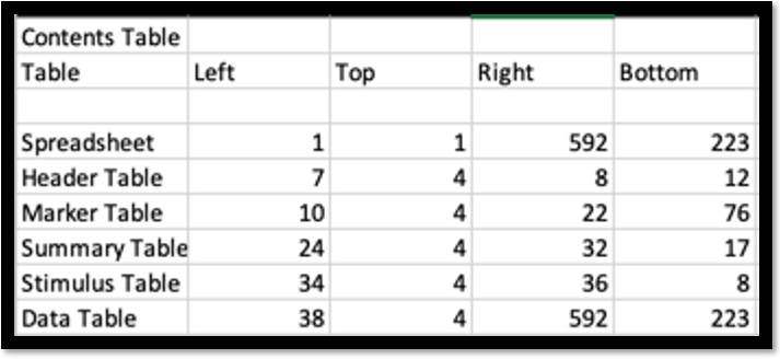
Contents table:  

A table of contents for all of the information provided within an export file; this table describes the location of the other tables in this file 

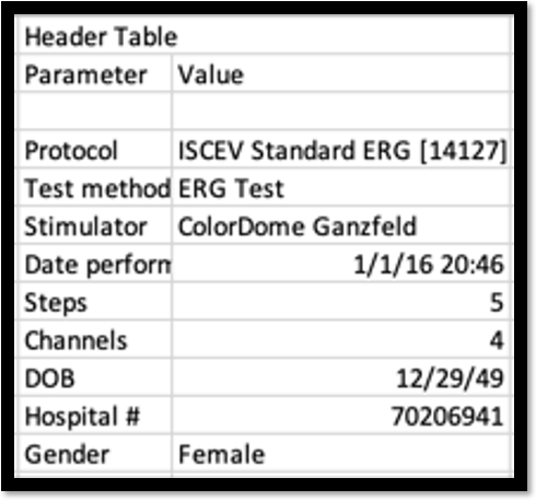
Header Table: 

Information about the patient and test 

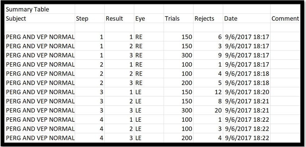
Summary Table:  

Summarizes the number of steps, results, trials, and rejections 

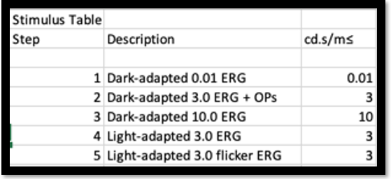
Stimulus Table:  

Stimulus parameters for each step of the protocol 

To export graphics:

1. From the main Export window, click on the Graphs button to move to the Graphs page. 

Click on any of the buttons to put a graphic of that information directly on your clipboard.

This will typically be the Graphs button. 

Note that graphs will be copied over in WSIWG format, that is, "what you see is what you get". If you wish to adjust graph layout options, add averages or remove artifacts, do that first!

Open the editing program of your choice and press "Paste". 

If you prefer to export to a file, toggle the "File" checkbox and press the Browse button. Navigate to the location and name your file. 

Important note: You must update the "save as type" field immediately below the filename input from text file to "All files", and you must use a suitable file extension (.bmp, .png, or .wmf recommended). 

Image Editing

If you place the file inside a Windows program such as Word, Excel, PowerPoint, or Wordpad, you can break the graphs apart into their component parts.

(Note that Image editing programs such as Photoshop or MSPaint are not able to do this.)

Insert the image into your document, then right-click on the image. Select either "Edit Image" or "Group > Ungroup" to devolve the image. 

You may see this notification: 

You can safely click Yes. 

Once the image has been converted  to a drawing object, you can adjust line weights and colors; delete unwanted graph elements such as backgrounds, or adjust font sizes.